Training transformers on real data often involves widespread repetition between data instances, which means the same tokens in the same order get encoded over and over again during training. This redundancy can happen any time that portions of prompts are reused, and it is particularly acute when training on data derived from simulated rollouts, such as in RL training of conversational agents, where initial trajectories often overlap. In these situations, the re-encoding of shared prefixes can dominate training time and memory consumption. We present a method for representing these shared prefixes as prompt trees and encoding them efficiently in a single forward pass of a standard transformer, computing correct gradients for all nodes in the prompt tree while only encoding each token once. On realistic data for training complex conversational agents, we show speedups of over 70x relative to training without prompt trees.

Overview

Consider a standard Reinforcement Learning (RL) setup for training a conversational agent. Given a prompt, a Large Language Model (LLM) is sampled many times to get a variety of rollouts. Each rollout is scored with some reward function, the prompt is duplicated for each rollout, and the whole group is batched together and passed to the forward and backward pass of a transformer-based model. This process wastes computation by re-encoding shared prefixes redundantly for each rollout. When those shared prefixes are short, the re-encoding is relatively inexpensive. However, when they are long, either because of complex instructions in a system prompt or a many-turn conversation prefix, this repeated encoding can become prohibitively expensive. The problem is compounded when doing simultaneous rollouts on multiple turns of the same conversation, leading to even more potential redundancy.

These kinds of shared prefixes exist not just in rollouts for conversational agents, but in many kinds of autoregressive transformer training. For example, when fine-tuning an LLM on a task-specific dataset, there is often a shared system instruction included before the training example. Any data that has any kind of implicit branching structure will have these shared prefixes, and they could even be mined from large collections of existing training data. Prefix caching exists as a known idea for handling shared prefixes at inference time, but there are as of yet no similar methods to improve efficiency at training time. We close that gap.

Shared prefixes in a prompt can be represented using prompt trees, a novel application of prefix tries that we introduce. A small example prompt tree is shown below:

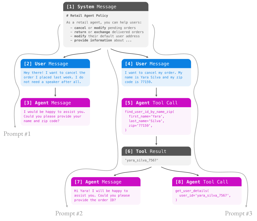
A prompt tree represents blocks of text in a prompt as nodes in a tree, where parent-child relationships encode whether one node’s text is immediately preceding another node’s text in the prompt. Considering again the RL example, rollouts that share a common prefix are represented as children of the node representing the end of that prefix in a prompt tree. In a multi-turn conversation, a rollout for one prompt typically becomes part of the next turn’s prompt, so the rollouts might themselves have children, with their own rollouts. For complex conversational systems, the depth and branching factor of these prompt trees can be large.

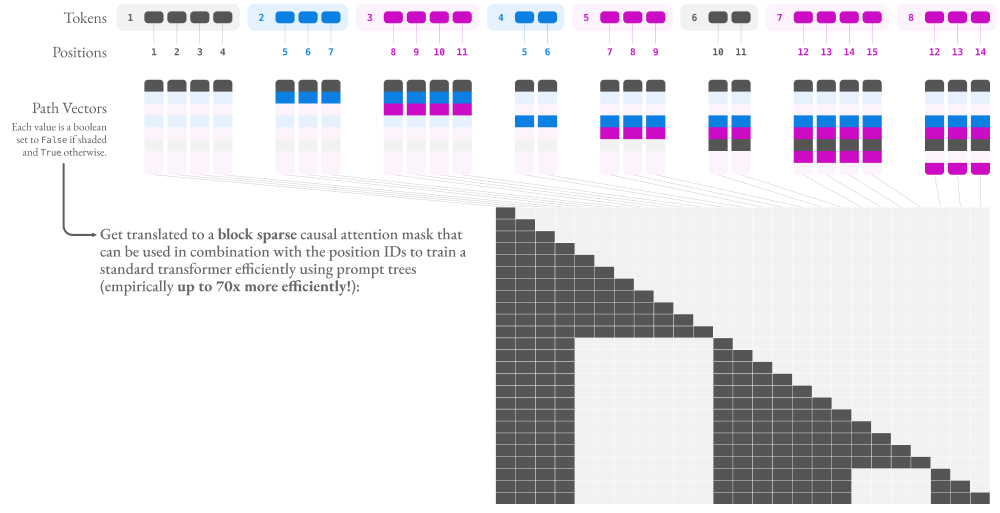
Our key technical contribution is showing how to efficiently encode a prompt tree with a single forward pass of a standard transformer. Each node in the prompt tree gets encoded once, but all tokens in all branches of the tree result in the same encodings and gradients as if they had showed up in a standard linear prompt representing the single path from the root of the tree to the node containing that token. We accomplish this non-redundant encoding by linearizing the tree to produce a flat sequence of tokens*Tooltip="The number of tokens in the flat sequence is equal to the sum of the number of tokens across all nodes."* and using a block attention mask that is computed from the tree structure, along with setting the position embedding for each token according to its position in the tree path (as opposed to its position in the linearized representation). This linearization enables training efficiently using prompt trees without requiring special kernels besides what is built into PyTorch.

Prompt trees can dramatically increase the efficiency of training, with the resultant efficiency gain increasing with the amount of shared prefix structure in the tree. To a first-order approximation, the efficiency gain should be linear in the amount of duplication that exists in the shared prefixes, though in practice we observe some variance from a strict linear relationship due to adaptive batching, tradeoffs between increasing batch size and increasing sequence length, imperfect sparsity in the block attention mask we construct, and other factors. On realistic multi-turn conversational data for complex agentic use cases, we observe speedups of over 70x compared to standard training setups.

Prompt Trees

A prompt tree captures the shared prefixes among many possible input sequences to a transformer. Each node represents some sequence of tokens, with edges between nodes capturing adjacency in the prompt. Nodes do not necessarily need to correspond to a semantically meaningful segments in a prompt, though they often do. Returning to the example application of rollouts in a conversational agent, nodes in a prompt tree would typically correspond to messages in a chat prompt. When constructing a prompt tree for RL rollouts, branching typically occurs after user messages, with multiple assistant messages or tool calls as children of a single user message. The figure we showed above was an example of a multi-turn conversation prompt, detailing the tokens included at each node (minus the chat message markup that would be in a final rendered prompt).

There are many ways to construct prompt trees, however, and the above image is just one such example. Below we show several other possibilities, including a densely-sampled collection of conversational rollouts, a prefix tree that is mined from plain-text prompts, and a trivial linear chain.

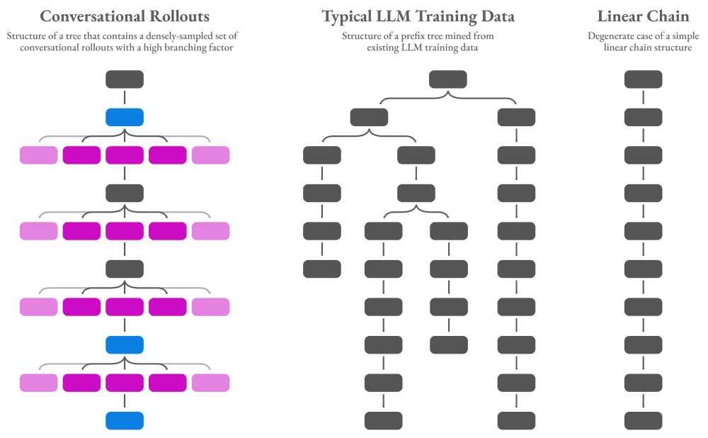
Different trees can have wildly different structures, and the amount of efficiency gain you can expect to see from using prompt trees is directly related to the structure of the tree. Each leaf node in the tree represents a unique prompt that would be a separately-encoded example in standard training setups. If we were to take all of the prompts in our toy example and encode them separately, we would get a collection of instances like this:

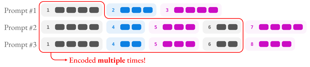
At a high level, you can take the prompt corresponding to each leaf node in the prompt tree and count its tokens, then compare the sum of all of those tokens to the sum of the tokens in the prompt tree. We call the ratio between these two sums the percentage of cached tokens in the prompt tree.*Tooltip="Note that by 'cached' here we do not mean tokens that are cached in the systems sense of the word, but rather conceptually cached in that we only compute their embeddings once and share them for multiple prompts in the same prompt tree, instead of recomputing them for each prompt as is done traditionally when training transformers."* The cached tokens are outlined in red in the figure above.

If we had a constant computational cost for encoding a single token, we would expect the speedup from using prompt trees to be proportional to the ratio of total tokens (including cached) to the number of tokens in a linearization of the tree, in terms of the overall FLOPS of the operations involved. However, the actual cost per token is not constant,*Tooltip="E.g., doubling the sequence length is typically more expensive than doubling the batch size, due to the quadratic complexity of the attention operation. Making that operation partially sparse, as we do, can help, but it does not completely eliminate the tradeoff."* nor is the implementation optimal (e.g., GPU memory access patterns are not currently optimized in our implementation), resulting in a sub-linear speedup. Even with those caveats, we empirically observe nearly linear speedups for typical model sizes and sequence lengths, as shown in our results below.

Training with Prompt Trees

Our goal is to encode the tokens of a prompt tree such that the resulting embeddings are exactly the same as what we would have obtained if we encoded each prompt (i.e., unique path) in the prompt tree independently using a standard autoregressive transformer. The key idea that we leverage is that when training an autoregressive transformer all tokens are encoded in parallel and their relative positions only affect two things: (i) the positional embedding of each token, and (ii) the causal mask used in the self-attention computation. Therefore, encoding a prompt tree simply requires proper handling of the position ID of each token as well as properly masking tokens in the self-attention mechanism.*Tooltip="This is conceptually similar to how Paged Attention (https://arxiv.org/abs/2309.06180) is used by vLLM (https://github.com/vllm-project/vllm) for prefix caching and chunked prefill at inference time. However, we cannot leverage paged attention here because we need to be able to back-propagate gradients during training. One approach would be to implement this naively using a dynamic computation graph but that would make batching challenging and would also result in an inefficient implementation."* We solve this problem by linearizing prompt trees and using a block sparse attention mask during training, resulting in an efficient implementation that requires no special kernels besides what comes built into PyTorch.

We define a tokenized prompt tree as \(\mathcal{T} = (\mathcal{N}, \mathcal{E})\), where \(\mathcal{N} = \{\mathbf{n}_i\}^N_{i=1}\) is the set of nodes in the tree and \(\mathcal{E} = {(s_e, d_e)}^E_{e=1}\), is the set of directed edges with \(s_e, d_e \in [1, N]\). Each node \(n_i\) is defined as a vector of token IDs for the corresponding prompt segment. Note that an important condition for our linearization process to be accurate is that the tokenization of the text in a prompt distributes across nodes in the prompt tree. That is, tokenizing the nodes in the tree and concatenating the resulting tokens needs to yield the same token sequence as concatenating the text of neighboring nodes and then tokenizing. This constraint is only relevant at the node boundaries, and when training chat models with nodes corresponding to messages, the tokenizers for most popular LLMs meet this condition.

Linearization, shown in the figure below, consists of converting a prompt tree \(\mathcal{T}\) into a linearized representation \(\mathcal{L} = (\mathbf{t}, \mathbf{p}, \mathbf{B})\) with \(S\) tokens, where:

• \(\mathbf{t} \in \mathbb{N}^{S}\) contains the flattened list of token IDs across all nodes based on a depth-first traversal of the prompt tree,
• \(\mathbf{p} \in \mathbb{N}^{S}\) contains the flattened list of position IDs that correspond to the tokens in \(\mathbf{t}\) (a position ID is defined as the position of a token in the path from the root node to the current node, assuming the token sequences of all nodes in that path are concatenated), and
• \(\mathbf{B} \in {\{0, 1\}}^{S \times N}\), contains a path vector of size \(N\) for each token in \(\mathbf{t}\). We define a path vector as a vector of size \(N\), the number of nodes in the prompt tree, where \(\mathbf{B}_{ik}\) is 1 if node \(k\) is in the path from the root node to the node that contains token \(i\), including the node of token \(i\), and 0 otherwise.

The vectors \(\mathbf{t}\) and \(\mathbf{p}\) are familiar concepts for training transformers, with minor variation for use with prompt trees. \(\mathbf{B}\) is novel. These vectors are useful because they offer us an efficient way to check if, for any two tokens \(i\) and \(j\), token \(j\) should be allowed to attend to token \(i\) (i.e., token \(i\) appears in token \(j\)’s prompt prefix). If token \(i\)’s path vector is a prefix of token \(j\)’s path vector, they are on the same path in the prompt tree. To compute correct attention, we further need to account for a causal attention mask for tokens that are in the same node, which we can do with the standard comparison of \(i \leq j\). We can compute the conjunction of these two conditions using an elementwise \(\mathtt{AND}\) (denoted as \(\land\)) between the two path vectors and comparing the result to the path vector of token \(i\), as follows:

$$\mathbf{t}_j \textrm{ can attend to } \mathbf{t}_i \overset{\mathrm{def}}{=} (\mathbf{B}_{i} \land \mathbf{B}_{j} = \mathbf{B}_{i}) \land (i \leq j)$$

Note that since \(\mathbf{B}\) only stores boolean values, we can represent it compactly by using 1 bit for each boolean value. This means that each path vector \(\mathbf{B}_i\) can be represented as a single value with at least \(N\) bits. If N is less than 64 we can use int64 values for this tensor. If there are more than 64 nodes in the prompt tree, we split the tensor into 64-bit chunks and do the \(\mathtt{AND}\) operation on each chunk sequentially.*Tooltip="Just-In-Time (JIT) kernel compilation is challenging with tensor reductions, so we use a loop with a fixed number of chunks per training run."* Our choice of path vector representation means that it is important to minimize the number of nodes in the prompt tree. So, while we have been describing nodes in the tree as corresponding to messages in a prompt, in practice we process the trees before linearization to collapse all linear-chain subtrees into single nodes.

This representation enables us to encode the linearized token sequence using a standard transformer, replacing the position IDs for each token with those in \(\mathbf{p}\) and using a block sparse attention matrix based on \(\mathbf{B}\), defined according to the equation above, such that the resulting embeddings are exactly the same as what we would have obtained if we encoded each path in the prompt tree independently using a standard transformer and a standard causal self-attention mask.

Given these three tensors, we can implement the appropriate attention mask efficiently using the Flex Attention module that is part of the PyTorch package. We do this by implementing a custom \(\mathtt{mask\_mod}\) function for Flex Attention that looks as follows (in pseudocode and referring to \(\mathbf{t}\) as \(\mathtt{tokens}\), \(\mathbf{p}\) as \(\mathtt{positions}\), and \(\mathbf{B}\) as \(\mathtt{path\_vectors}\)):

# Legend:
# B: Batch size.
# S: Sequence length.
# C: Number of 64-bit integer chunks used for representing path vectors.
# tokens: Integer tensor with shape [B, S].
# positions: Integer tensor with shape [B, S].
# path_vectors: Integer tensor with shape [B, S, C].
def prompt_tree_mask_mod(
  b: torch.Tensor , # Integer scalar representing the batch index.
  h: torch.Tensor , # Integer scalar representing the hidden index.
  q: torch.Tensor , # Integer scalar representing the query index.
  kv: torch.Tensor , # Integer scalar representing the key-value index.
) -> torch.Tensor:
  q_path = path_vectors[b, q]
  kv_path = path_vectors[b, kv]
  has_shared_prefix = q_path[0].bitwise_and(kv_path[0]) == kv_path[0]
  for c in range(1, C):
    has_shared_prefix = (has_shared_prefix
      & q_path[c].bitwise_and(kv_path[c]) == kv_path[c])
  causal_mask = q >= kv
  return has_shared_prefix & causal_mask

Flex Attention takes this \(\mathtt{mask\_mod}\) function implementation and compiles it into a Triton self-attention kernel. The resulting kernel has performance characteristics that are similar to Flash Attention, meaning that training with prompt trees has similar step times and memory consumption to standard transformer training, while being able to pack a lot more information into each batch. The binary encoding of paths into path vectors leads to a very efficient \(\mathtt{mask\_mod}\) computation—when running training with equivalent sequence lengths, and prompt trees that need up to 4 chunks in their path vectors, we observe step times that are only a few percent slower than training using FlashAttention.

Results

How well does this work? Below we show the speedups that we see for training a standard transformer on some of our internal data, where we construct prompt trees with varying percentages of cached tokens. Training is performed on a cluster of Nvidia H200 GPUs, using an adaptive batching strategy that groups instances together into variable-sized batches according to their length in order to saturate the GPU memory utilization as much as possible.

In the figure below, the \(x\) axis shows the ratio of cached tokens to real tokens in the prompt tree. The specific metric on the \(x\) axis is the number of unique tokens plus the number of cached tokens divided by the number of unique tokens (i.e., if all tokens are unique, the "cached token ratio" is 1). The far left of the figure corresponds to trivial (linear chain) prompt trees, and the trees get progressively more branches and more deep as the ratio of cached tokens increases. The \(y\) axis shows relative speedup compared to making separate instances for each path in the tree. We specifically compute the time to finish a single epoch over the data both with and without prompt trees and show the ratio on the \(y\) axis.

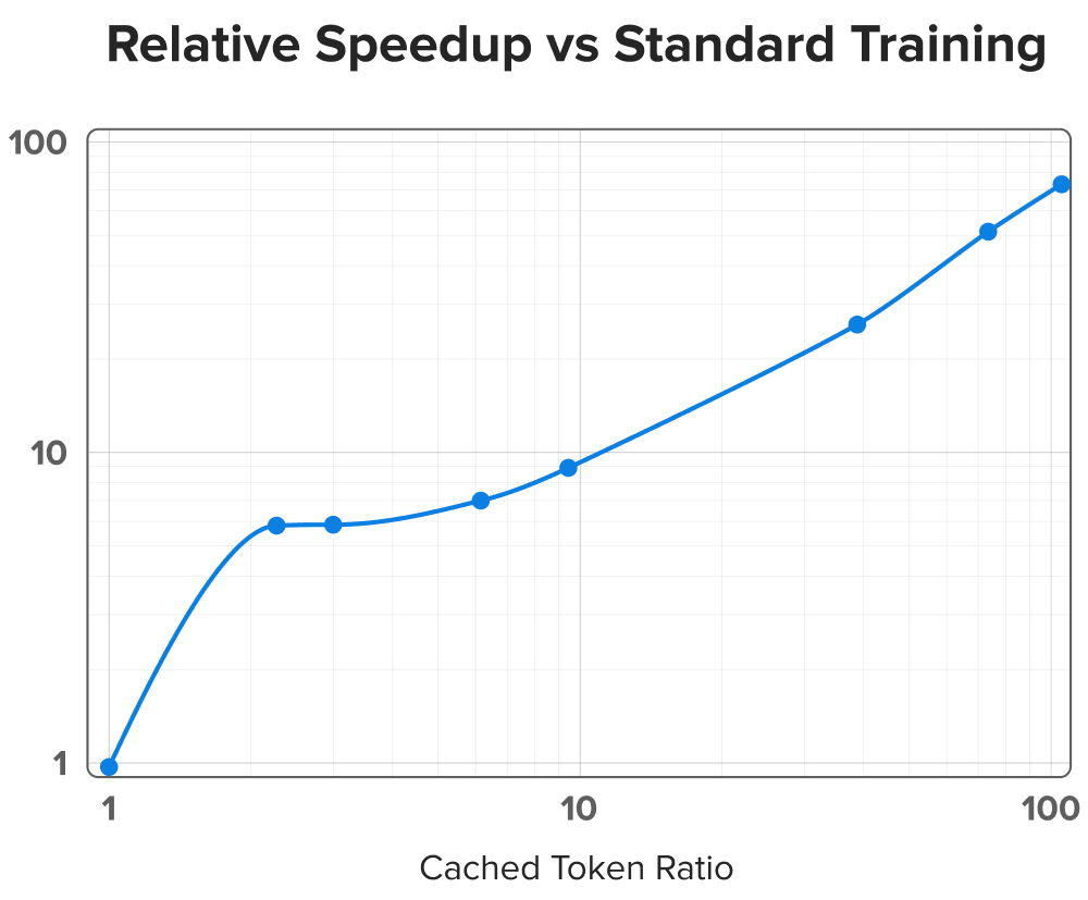
The above plot shows a roughly linear relationship between the ratio of cached tokens to prompt tree tokens and the observed speedup, with a maximum speedup using our data and GPUs of over 70x. This proportionality means that the upper bound for speedups is largely dependent on how many tokens can fit in GPU memory, along with how much branching can be meaningfully made use of in a single tree. If you have a means of packing prompt trees arbitrarily densely in an informative way, and GPUs that can fit very long sequences, you could likely achieve higher speedups than even the 70x that we have shown.

However, the actual speedup we see is not exactly linear. As the prompt trees get larger, several factors combine to reduce the speedup: the difference between encoding a very long sequence and batching together many smaller sequences,*Tooltip="We are not increasing the number of non-masked tokens attended to for any token in any input. If we were able to align kernel blocks (where block sparsity is computed) with prompt tree nodes perfectly, the extra quadratic penalty for increasing the sequence length in prompt trees would be negligible. Prompt tree nodes are variable size, however, so getting perfect block alignment is challenging."* the need for more chunks in the path vectors that slows down the mask mod computation, and other practicalities of adaptive batching strategies (it gets harder to completely fill a GPU as the instances get above half of the token limit). Together these factors mean that we only get a ~70x speedup when the cached token ratio is ~100. On the other hand, at lower cached token ratios, we often see higher speedups than the ratio; this is due again to the particulars of adaptive batching and exactly how many instances can fit on the GPU at each step. Finally, to measure the slowdown produced by using the flex-attention-based prompt tree encoding instead of flash attention, when we remove all cached tokens from the prompt trees, we see a relative speedup of 0.97, meaning that there is a 3% penalty induced by the prompt tree attention implementation.

Limitations

As we showed in the previous section, training with prompt trees can lead to dramatic speedups in terms of time to make a full pass over a dataset. This is not necessarily the same thing as time to convergence in a training run, however. If the loss is only computed over leaf nodes in the prompt tree, then the gradients computed with prompt trees and with standard transformers will be identical. Most RL training would typically only compute a loss on the leaves, so what we showed is a reasonable estimate of potential speedups for RL training. However, if there is also a loss on internal nodes of the prompt tree, this could get a different weighting in the optimization if care is not taken to account for the number of paths the internal nodes participate in. That is, if an internal node would have shown up with a loss in 20 examples in a standard transformer, that node will only have 1/20the weight in the optimization with prompt tree training. This difference is easy to account for with token loss weighting if desired, though increasing the weight of a token in a single batch may not have the same effect on optimization as seeing the same token 20 different times in different gradient steps spread throughout training.

Another potential issue when trying to go from training step speedups to convergence speedups is the effective batch size. Prompt trees let you increase the effective batch size relative to standard transformer training by an order of magnitude or more, but it could be that increasing the batch size does not improve optimization, or that using prompt trees decreases the diversity of examples in a batch in a way that negatively impacts optimization. Prompt tree training is most obviously beneficial when you are already doing multiple gradient accumulation steps to increase your batch size, and you have many GPUs that can each compute gradients from different prompt trees.

Lastly, while we've largely focused our exposition on RL training, computing gradients is only one part of the inner loop of that training. We do not speed up the time for on-policy sampling, which is another large part of that inner loop. Our method is applicable for computing gradients with any tree-structured data, however. RL training of LLMs is a common application that results in tree-structured data, but it is not the only one.

Conclusion

Repeated subsequences across examples are common in many kinds of data that standard transformers are trained with, especially when performing RL rollouts of multi-turn conversational agents. We have shown how to dramatically increase the efficiency of transformer training in the presence of repeated subsequences using prompt trees, a method that can be thought of as prefix caching at training time. On realistic prompt trees constructed from real conversational agents, we have shown that prompt tree training results in speedups of more than 70x. Even higher speedups than this can likely be achieved with careful thinking about how to optimize data collection to fully make use of prompt trees, in many more domains than RL training with conversational agents.